In late January 2022, Argonne National Laboratory partnered with University of Chicago, National Center for Supercomputing Applications, and NVIDIA to host the AI Hackathon in Molecular Dynamics, a student competition focused on using AI to develop creative solutions to modeling and simulation challenges in molecular dynamics. Argonne recently announced our win!
This project perfectly embodied my goals for grad school:
- Solve a thorny scientific problem with novel, creative, applications of ML.
- Enjoy a cross-functional team of scientists: experts in material science, polymers, math and computer science, where I was able to serve as the AI specialist.
- Work with super-compute hardware. ThetaGPU has 192 A6000 GPUs across 24 nodes. Each node has either 320GB or 640GB (!!) of GPU memory to train Very Large Models, and, crucially, the high-capacity networking InfiniBand (!!) to make that scale useful.

My wonderful heterogeneous team of scientists:
- Aria Coraor – Molecular Engineering, de Pablo Group, PhD @ UChicago.
- Ruijie Zhu – Computer Science, MS @ Northwestern University.
- Seonghwan Kim – Material Science, PhD @ UIUC.
- Jiahui Yang – Material Science and Engineering, PhD @ Northwestern University (not pictured).
- Me, Kastan Day – Applied Machine Learning, MS @ UIUC.
Problem Overview
The problem is to predict how molecules of plastic (polymers) structure themselves when left to settle into equilibrium. We used molecular structure to predict the “period” at which these layers repeat.
This is well characterized for short chains of molecules but becomes more difficult as (1) molecules get longer and (2) as the number of types of molecules in the chain increases above 2. In this competition the polymers were always 64 sequences long and had 2 or 3 types of molecules.
Our input is a string representing the polymer chain: “AAABCCBBBCC” of length 64. There is also an “interaction parameter” which characterizes how strongly B-C molecules are repelled from each other, it is a floating-point number between 0 and 3.5.
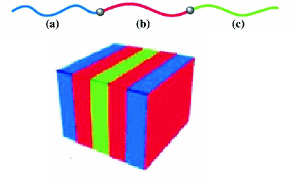
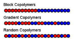
Our output is a float number between 0 and 16, representing the length of the Lamellar period shown in these diagrams.
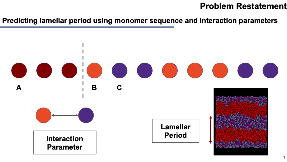
These visuals further lend intuition about the problem space. We’re working with polymers that are a “block” of “A molecules” for the first 32 positions, then they’re random for the remaining 32 positions.
Our solution
I loved trying to understand the polymer’s key properties from the domain-experts on our team. Then I attempted to translate these key ideas into a ML model that attends to the proper features. What’s the right model to use?
At first, since this is a “structured data” problem (not using images or audio), I thought XGBoost would be the most successful model. My prior research on which algorithms win in the real world shows that XGBoost dominates all structured data problems, while deep learning is more successful against “unstructured” data. However, the data has long-range dependencies that are not well captured by decision trees.
Next, I tried using Transformers since Attention would capture long-range dependencies. These occur when the polymer molecule’s tail “wraps around” and interacts with other parts of the molecule. However, attention is overparameterized, we have little data in this challenge and the model did not converge during training.
Finally, I tried transforming the molecular since problem into an image problem and used a CNN. Delightfully, this creative solution ended up providing the best results.
- CNN
- Kernel Machine
- Auto-encoder
But the CNN can’t capture long-range dependencies! Enter feature engineering, a crucial step for most real-world problems.
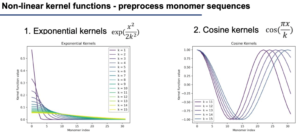
We created a set of new inputs by feeding them through exponential kernels (to capture long-range dependencies) and cosine kernels offset by different amounts (to capture long-range dependencies that occur mid-polymer-sequence). These features introduce new non-linear features that allow the model to see a fuller picture.
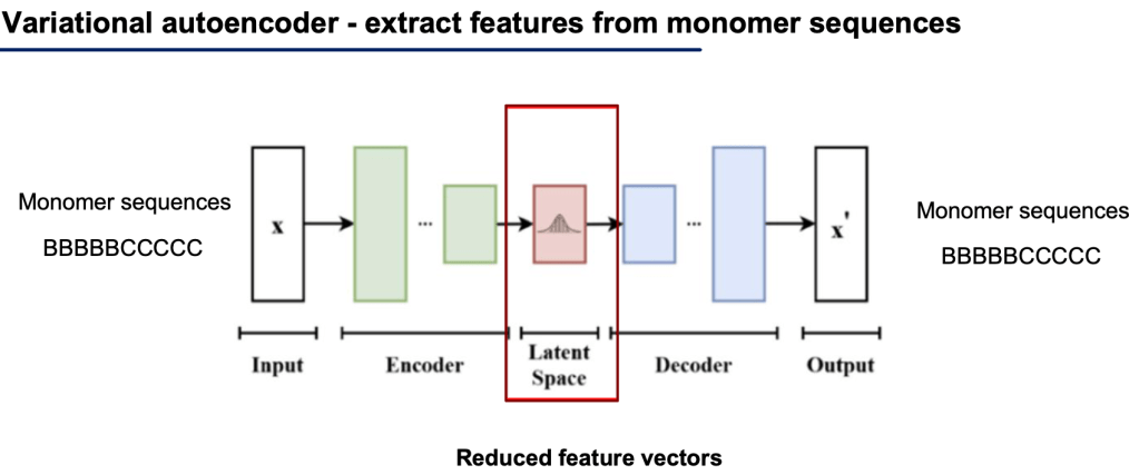
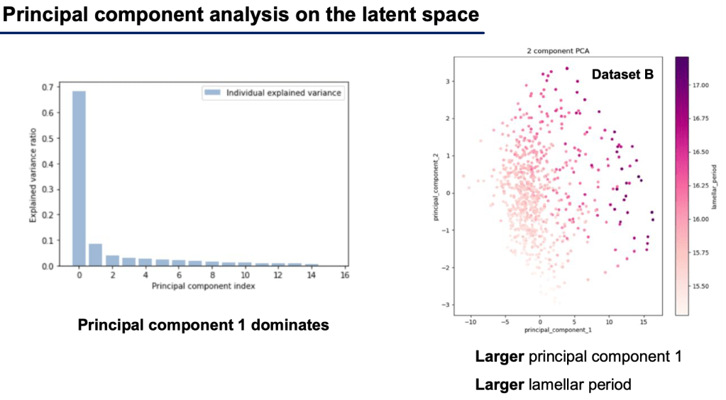
Additionally, we used a standard Autoencoder to provide additional non-linear features to the model. After training the model, we simply run the model over all our input sequences and extract the latent space (red box below) for each input sequence, and directly use that (lower-dimensional) vector as input to our final model.
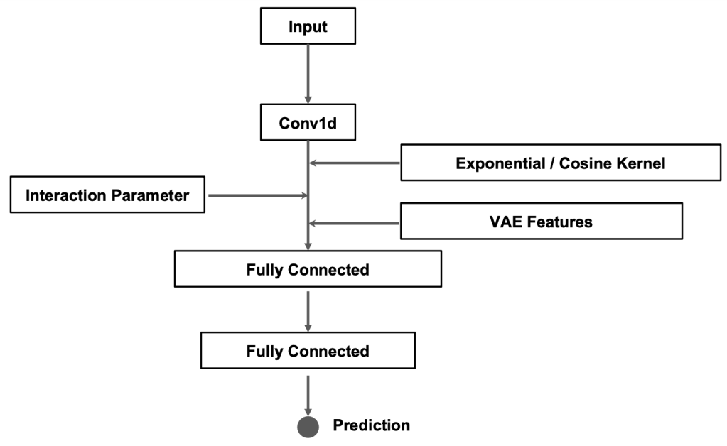
Finally, our model is built by running a CNN on the input sequence, then feeding the other feature-engineered values into the fully connected layers. This allows the fully connected layers to equally evaluate the inputs from each form of feature engineering to finally produce a final regression prediction of the lamellar period.
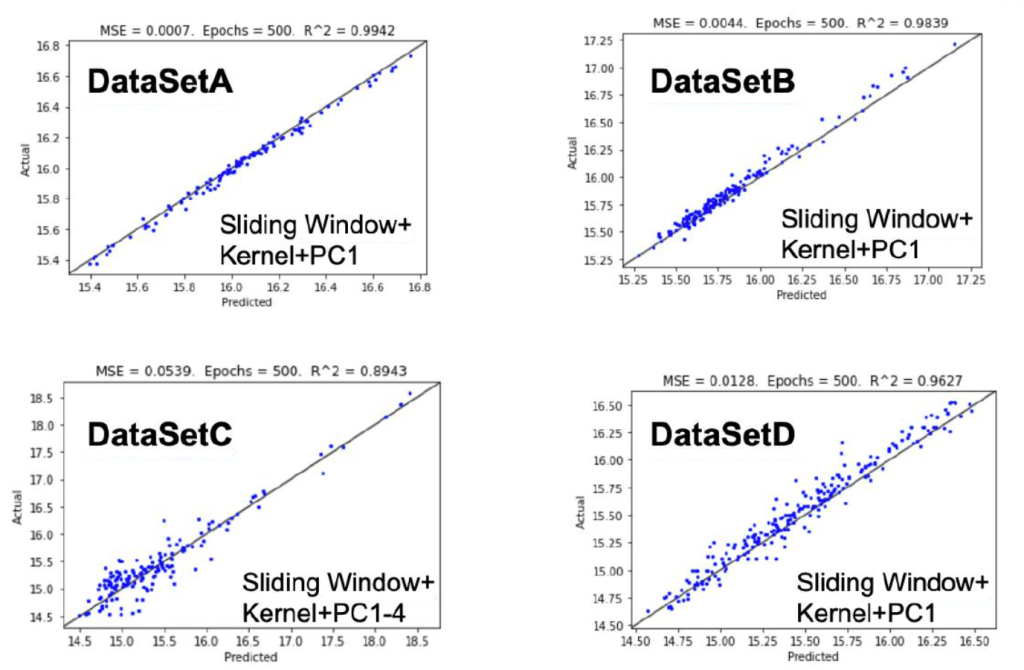
Results
Ideally, we would see all blue points fall exactly on the 45˚ Y=X black line. That would mean that each predicted value is exactly the same as the ground truth (“actual”) value.
Explainability
Deep learning is notoriously difficult to explain. In our early data exploration, I used XGBoost to product “feature importance” values for each element of our input. Discovering which elements of our data explain our predictions will help up design the right model for the task. Furthermore, it helps molecular scientists better understand these interactions, so they can develop new hypotheses to test.
I was surprised to find that position 24 of [0-31] total positions had the greatest explanatory power, even more than the interaction parameter. Furthermore, it was interesting that the ‘tail’ of the sequence was the 2nd most critical area.
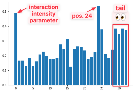
The first value (from the left) is ‘magnitude/interaction’ param.
Top 3: (’24’, 0.537), (‘mag’, 0.490) (’30’, 0.383).
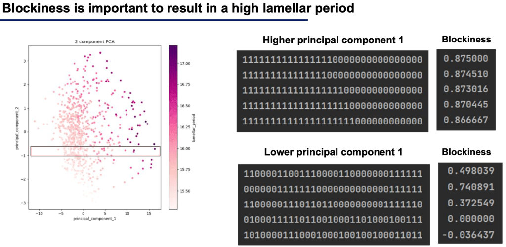
Another important finding was that greater blockiness means greater lamellar period. We observed this after a qualitative analysis of the principal components of the latent space of our ML model.
So we can see our model is able to predict our finally output, a regression score of lamellar period and this is evident in the PCA of the model weights, “the hidden space activations,” shown below.
Competitor’s solutions
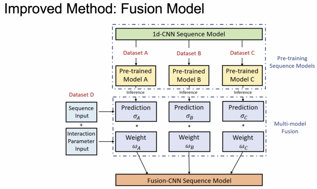
I’d like to highlight another team’s work. They had an elegant solution of training a CNN model on each of the individual datasets then ensembling their predictions together via a weight value that was learned by the model. Model ensembles are common, but I like the idea that the weight parameter was learned, instead of human-determined.
If you enjoyed this post, read my other machine learning posts on kastanday.com